This post will explain how to use the tracker sheet and my ES sheet.
On the Tracker sheet in cell G1 is the date that will be used if you click Track Select (cell C1) or Track Spread (cell D1). If you have the risk file for last Friday downloaded and in your C:\Span4\Data folder then put 20151218 in cell G1.
On the Tracker sheet I have listed in row 3 a naked short option ESh6p1650. The Net column has a -1 meaning one short
contract. Positive numbers in the net column are for long options.
The number 1 in the S1 column is for grouping strategies. This naked option is in group 1 without any other options.
In row 4 I have the same short option and in row 5 I have two long ESh6p1350 options.
The number 2 in the S1 column for rows 4 & 5 tells the program to combine them together as a spread.
Click on Clear Hist Data in cell N2 to clear the HistData sheet.
If you select cells A3, A4 & A5 and then click Track Select (cell C1) you should get this.
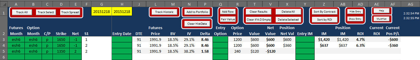
Row 3 shows $1,420 IM for the naked option.
Row 4 shows $637 IM for the spread.
The HistData sheet shows the raw data for what you just calculated. I added columns AI to AP to the original excel so that more calculations could be done to the data.
(Note I have had trouble with getting results on the HistPivot sheet if cell AI1 is blank. That usually happens when I change
contracts on the Tracker sheet. If the data on the HistPivot sheet didn't update then check to see if there is a number in cell AI1. If not the put a number in this cell and then on the HistPivot sheet right click on any data that is there now and the left click on Refresh.)
To run historical research on an option or spread
- Go to Tracker sheet
- Put the starting date (format YYYYMMDD) in cell G1. Use one trading day before you are adding the position. So if you want the position to start on 11/30/15 then put 11/27/15 in cell G1. The reason for this is that when you are looking to add a position today the IM you will have is the IM from the prior trading day.
- In cell H1 put the ending date for the research.
- Click on Clear Hist Data in cell N2 to clear the HistData sheet.
- Left click cells A3 and then hold the left click and drag down to cells A4 & A5 so that all three are selected.
- Click Track Historic in cell L1.
- You can now watch the program go through each day calculating all of the data. All of this data will be on the HistData sheet.
- Go to the HistPivot sheet. It is actually a Pivot Table. It should look like this.
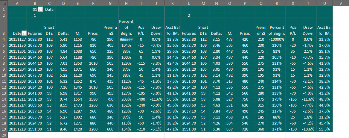
- Column A has the dates. Row 2 has the numbers you put in column S1 on the Tracker sheet. Columns B-K have the data for the option that has "1" in column S1 on the Tracker sheet. Columns L-U have the data for the spread that has "2" in column S1 on the Tracker sheet.
The first 6 columns (B-G for number 1) for each S1 number have raw data. The next 4 columns (H-K for number 1) have calculated data. This calculated data is not quite correct if you are using the first date for the day prior to the day you are adding the position. That is why it is best to move it over to the ES sheet.
- To move this data to my ES sheet that shows some additional info you would copy the date column from HistPivot and paste it to the first column in each block on the ES sheet. You would then copy the raw data (for number 1 in this example cells C4 to G19) and paste it to cell B5 using Paste Values. Copy raw data in cells L4 to Q19 for number 2 to cell S5.
- Put the positions in the green cells in rows 2 & 3 columns C thru F on the ES sheet. The column F that has the number of positions is important so that the MROI can know how many contracts are in the position to correctly calculate fees.
- In cell A1 of the ES sheet you should enter your total round turn cost per contract.
- In cell B1 you should enter the multiplier for your IM. If you are using IMx3 then the number 3 should be in this cell.
the ES sheet should look like this
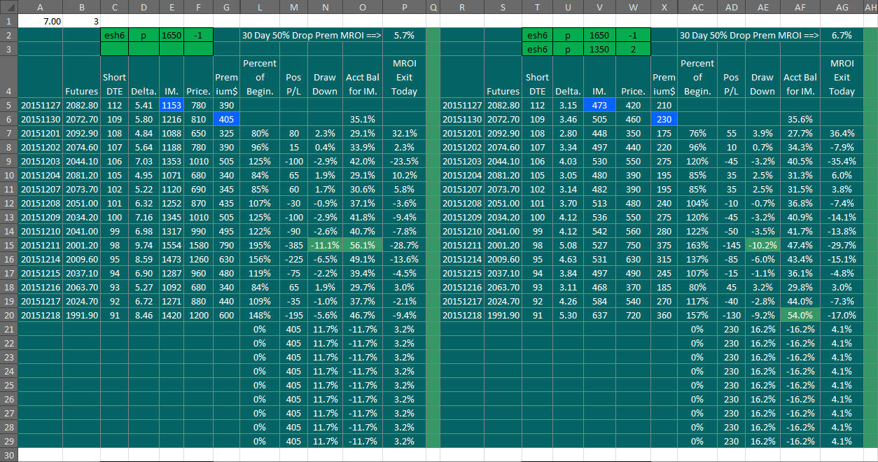
The blue cell E5 is the IM used for that block to do the calculations.
The blue cell G6 is the
premium used for that block. This is the settlement. If you want you change this to what you actually entered a trade at you can do that here.
There are some hidden columns to make calculating easier. Normally you do not need to see what is there.
Column L or Percent of Beginning is current Premium in dollars divided by beginning premium.
Column M or Pos P/L is profit or loss in dollars since starting the position. It does not include costs.
Column N or Draw Down is Pos P/L divided by (beginning IM times the number in cell B1). A negative number means that the position has lost money since it was started. Positive is a profit. Again these are gross not net numbers. Costs aren't included. I have the lowest number in this column turn to a green background fill.
Column O or Acct Bal for IM is (Current IM + (Pos P/L*-1)) / (Beginning IM * number in cell B1). This percent, if this was the only position you had on and you fully invested in this position, would be how much of your account was now being used by IM. When this number goes over 110% you are on
margin call. (You don't go on margin call until the maintenance margin is gone. Maintenance margin is 10% less than IM). I have the highest number in this column turn to a green background fill.
The blocks on the ES sheet can be copied and pasted to other areas of this sheet or to other sheets. If you need more lines per block then insert more lines and then copy down all cells from the last line of the block into the new added lines. This should keep the cell highlighting correct.
I hope this is clear.